Choosing a measure

SPINE cuts a nonnegative measure into scale strata. It does not know what that measure means. Choosing it is the modelling step, and it decides what question is being asked, more than any other decision made with this method.

The structure SPINE finds is a property of the pair: the objects, and the quantity by which they are compared. Change the quantity and the same objects can separate differently, or not at all. This page is about making that choice deliberately. It assumes the construction is already familiar.

1. What a measure has to be

Formally, a measure is a map from the objects to the nonnegative reals,

μ : 𝒪_{N} ⟶ ℝ_{+}, m_{i} = μ (o_{i}) \geq 0,

(1)

finite, one value per object. Those two requirements are mechanical and are checked for you. The third is the substantive one and cannot be checked by any software.

The measure must be on a ratio scale

Every quantity SPINE computes depends on the measure through the normalized prefix shares, which are ratios. The method therefore reads multiplicative separation: it asks whether one group of objects sits at a different scale from another, and different scale means a ratio. For that question to mean anything, zero must mean none of the thing, and $8$ must mean twice as much as $4$ .

Counts, distances, energies, frequencies, degrees, magnitudes, concentrations and durations all satisfy this. Quantities whose zero is a convention do not:

Temperature in °C or °F. Twenty degrees is not twice ten degrees.
Calendar dates and years. The same problem.
Signed z-scores and anomalies. Zero means average, and values go negative.
Log-transformed quantities. The log's zero is the original's one.
Correlations, or anything on a fixed −1 to 1 range. No meaningful zero.

Most of these have an easy repair: take a magnitude, or a distance from a declared reference. $| T - T_{ref} |$ is a valid measure where $T$ is not, and $| z |$ is valid where $z$ is not. The repair is a modelling statement in itself, because it declares what counts as none of the thing.

2. Validity is not usefulness

A valid measure still has to carry the structure being looked for, and carry it multiplicatively. If it does not, the incremental nested entropy profile rises and never turns over, and SPINE returns one unresolved stratum.

A single stratum is an answer. It says this measure does not separate these objects into scales. That is a property of the measure that was chosen, not of the cut, and it is a different statement from “these objects are all alike”. The remedy is a measure that expresses the structure better, not a looser setting; there is no setting to loosen.

3. The measures, and what each makes an object

Four of the ten change what an object is, which changes how many objects there are and what a stratum means. That is worth checking before anything else.

Measure	Value for object $i$	An object is	Usual orientation
`asis`	a quantity you already have	a row	yours
`dist2mean`	$‖ x_{i} - \bar{x} ‖$	a row	upper
`dist2median`	$‖ x_{i} - \tilde{x} ‖$	a row	upper
`zrownorm`	the same, features scaled by their standard deviations	a row	upper
`robustrownorm`	the same, features scaled by their MADs	a row	upper
`knn`	distance to the $K$ th nearest neighbour	a row	upper
`frequency`	$n_{i} / \sum_{j} n_{j}$ , counts supplied	a category	lower
`statefrequency`	the same, counts tallied for you	a distinct state	lower
`degree`	$\sum_{j} A_{i j}$	a node	upper
`singular`	$σ_{i}$	a singular value	upper

For singular, the objects are the singular values themselves, so their number is the smaller dimension of the matrix rather than the number of rows. For frequency and statefrequency, the objects are categories or distinct states, so forty thousand observations over three distinct states give SPINE three objects, which is not enough to partition. A rich state space is needed, not merely a large sample.

The choice between those two is only about what is already held: one count per category already tallied, or raw observations still to be tallied. Rows are matched exactly and at full binary64 precision, so two rows are the same state only when they agree bit for bit; rounding or binning first is a modelling decision about what counts as the same state.

Where to start

If the domain already hands you the number — a firing rate, a claim size, an energy, a residual magnitude — use it and stop. A domain quantity almost always beats a constructed one, because it carries meaning the reader already has. Otherwise the question is what would make an object notable, and the two common answers are not the same question, which is the subject of section 5.

4. Orientation

The measure gives an ordering; the orientation says which end of it is the atypical one. It is a scientific claim about the problem, not a display setting. Upper for distances, degrees and energies, where large is the departure. Lower for frequencies, where the rare tokens are the interesting ones. Bilateral when both ends are atypical, naming an anchor object that sits in the typical middle, after which scores measure separation from the anchor's stratum in either direction.

Getting it backwards does not produce an error. It produces a confident answer to a question that was not asked.

5. Distance is not density

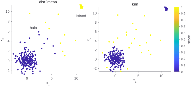
This is the commonest way to choose the wrong measure, because the two questions sound alike in words and are unrelated in the data. Consider three planted groups in the plane: a bulk, a halo displaced a little and spread widely, and an island displaced a long way and packed tightly.

Two scatter plots of the same points coloured by score. Under dist2mean the tight island at the top right is the darkest thing in the picture. Under knn the same island is as pale as the bulk and the diffuse halo is dark instead. — **Figure 1. The same objects, two defensible measures, opposite answers.** Left, distance from the mean: the island is maximally atypical, scoring 1, together with the outermost halo points. Right, distance to the fifth nearest neighbour: the island scores exactly 0 — perfectly typical — and the sparse halo is flagged instead. Neither is wrong. The island is far away *and* densely packed, so its neighbour distances are small.

Distance from a centre and local sparsity are different properties, and the measure is where the analyst says which one was meant. When the answer matters, running both and comparing what each flags is cheap: agreement means the structure is robust to how the question was asked, and disagreement is telling you something real about the data, at which point choosing between them is a scientific decision made deliberately rather than by default.

6. Do not standardize by a statistic the far objects inflate

Both row-norm measures compare an object with a centre after putting the features on a common footing, and differ only in the statistics used:

μ_{i}^{z} = \sqrt{\sum_{f} {(\frac{x_{i f} - {\bar{x}}_{f}}{σ_{f}})}^{2}}, μ_{i}^{robust} = \sqrt{\sum_{f} {(\frac{x_{i f} - {\tilde{x}}_{f}}{{MAD}_{f}})}^{2}} .

(2)

Standardizing at all is usually necessary: a row norm over metres and kilograms is dominated by whichever unit produces larger numbers, and the partition then reflects a choice of units rather than anything in the data. But the scaling statistic matters, because when objects at a far scale are present they inflate the standard deviation that is about to be divided by, compressing everything below them.

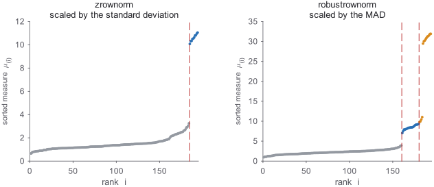
Two panels of the sorted measure against rank for the same eight-dimensional data. Under zrownorm the middle group is not separated from the bulk and there are two strata. Under robustrownorm three strata appear. — **Figure 2. The same objects, standardized two ways.** Three planted scales in eight dimensions, asked the same question. Scaled by the standard deviation, the middle scale is compressed into the bulk and two strata are returned, of 184 and 10 objects. Scaled by the median absolute deviation, which the far objects do not inflate, three strata appear, of 160, 20 and 14. The dashed lines are the cuts.

When hunting for objects at a different scale, prefer the statistics those same objects do not distort: robustrownorm over zrownorm, and dist2median over dist2mean, unless there is a reason not to.

7. A transformation of the measure is a different measure

Multiplying a measure by a positive constant changes nothing, because every normalized share is a ratio. A nonlinear monotone map is not in the same category:

μ ⟶ c μ changes nothing; μ ⟶ φ (μ) changes the analysis.

(3)

Order is preserved by both, but only the first preserves the ratios. A squaring stretches the separation between scales, a logarithm compresses it, and the entropy geometry moves accordingly.

Figure 3. One quantity, three measures. The same 168 objects under the raw measure, its square, and

\log (1 + μ)

. Squaring moves the cut by seven objects; the logarithm compresses the separation until there is no transition left to cut on. None of the three is a display choice.

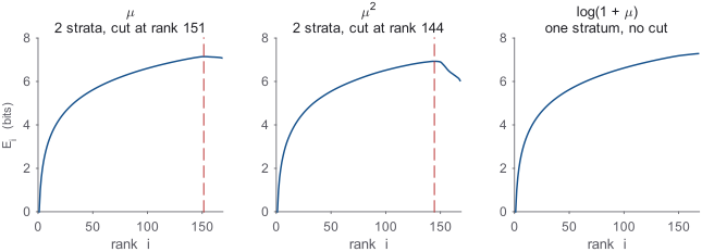
So a transformation applied to make a plot look better is not cosmetic here. It has to be justified as the measure it now is.

8. A bounded measure has to be inverted

The profile turns over when an incoming value is large against the mass already accumulated, and that comparison is made through the incoming fraction

q_{i} = \frac{m_{(i)}}{S_{i}} .

(4)

A measure confined to $(0, 1]$ — a bottleneck ratio, a coverage fraction, a normalized cost — caps $m_{(i)}$ at exactly the end where the interesting objects sit, so $q_{i}$ can never get large and the profile never turns over. If small values are the extreme ones, invert first and read the result upward.

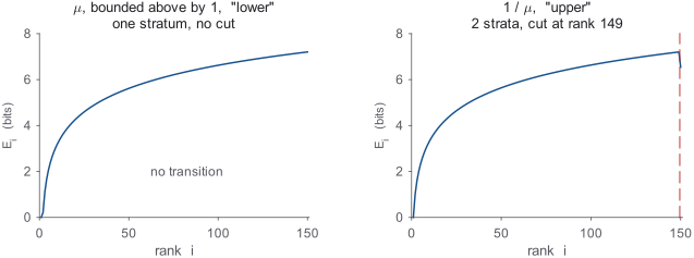
Figure 4. The extreme end needs room to separate. One value sitting far below all the others. Read as a bounded ratio, the profile never turns over and there is one stratum. Read as its reciprocal, the same value has an unbounded end to occupy, the transition appears, and it is separated.

The general rule: SPINE reads multiplicative separation, so put the extreme end of the measure where it has room to separate.

9. Practical notes

Ties are information

No boundary may fall inside a block of equal measure values, so objects the measure cannot tell apart always share a stratum. A heavily quantized measure — integer counts, rounded instrument readings — therefore admits few boundary locations. That is deliberate rather than a limitation to work around.

Constant and mismatched features

A feature with no spread carries no information about differences between objects. Features in different units, left unscaled, hand the partition to whichever unit produces the larger numbers.

Very large collections

The profile is evaluated in binary64, with its accumulated summation error checked against an independent closed form, and a profile whose error cannot be resolved is declined rather than approximated silently. The tolerance tracks the error's own growth with the collection, so fields of over a million values resolve routinely, and a refusal reflects an extreme dynamic range in the particular values rather than their count. When one does occur, the remedy is built in and deterministic — the cut is located on a thinned copy of the sorted measure, which is a quantile subsample and preserves the shape of the distribution, then applied to every object. Subsampling at random instead would move the located cut with the seed.

Scores travel, cut values travel further but only in context

Scores are always 0 to 1, so two analyses can be compared directly. The measure value at a cut is in the units of your own measure, which makes it the quantity to quote in a paper and to apply to new data — but only against the same measure, since it means nothing under a different one.

10. If you are unsure

Take two measures that encode genuinely different questions, a distance one and a density one, and look at both. If they agree, the structure is robust to how it was asked. If they disagree, as in section 5, the disagreement is a finding about the data, and choosing between them is a scientific decision you are now equipped to make deliberately.