SPINE — Scale Partitioning by Incremental Nested Entropy

A collection of objects carries a nonnegative measure: a distance, an energy, a count, a degree, a singular value. SPINE asks where that collection separates into distinct scales, and how strongly. It is not told how many groups to look for, and it has no detection threshold to set.

Two things are supplied, and they are the scientific input. A measure, one nonnegative number per object, saying what the objects are being compared by. An orientation, saying which end of that measure is the atypical one. Everything after them is computed from the measure alone.

Implementations

MATLAB Reference implementation. User guide, function reference, conformance fixtures. Python pip install entropy-spine. User guide, function reference, the same conformance fixtures.

R Planned against the same specification. Not yet implemented.

The three are not three methods. A language-independent specification fixes the computation, and a shared set of conformance fixtures and expected outputs decides whether an implementation agrees with it. The MATLAB package is the reference; the Python package is verified against the same fixtures, exactly; R is stated here as intent.

The construction

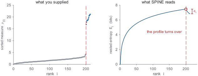
Let the objects be $o_{1}, \dots, o_{N}$ and let the measure give them masses $m_{i} = μ (o_{i}) \geq 0$ . Sort them, so that $m_{(1)} \leq \dots \leq m_{(N)}$ , and walk up that order. At rank $i$ , the objects admitted so far carry a total mass and a share of it each:

S_{i} = \sum_{j = 1}^{i} m_{(j)}, p_{j}^{(i)} = \frac{m_{(j)}}{S_{i}} .

(1)

This probability is measure-induced. It is the fraction of the accumulated measure carried by each object admitted so far, and it is an occurrence probability only when occurrence frequency is itself the chosen measure. Evaluating the Shannon functional on that nested family of prefixes gives the incremental nested entropy profile:

E_{i} = - \sum_{j = 1}^{i} p_{j}^{(i)} \log_{2} p_{j}^{(i)}, E_{i} = 0 when S_{i} = 0 .

(2)

The profile is one number per rank, and its shape is the whole object of study. While objects of one scale are being admitted, each new one genuinely adds to the spread and the profile rises. When an object arrives from a multiplicatively larger scale, it dominates everything below it: the normalized mass concentrates rather than spreading, and the profile turns over. That turnover is the cut.

Figure 1. The turnover is the cut. Two hundred objects drawn from one scale and twelve from a far larger one, measured by distance from the mean. Left, the sorted measure. Right, the profile that SPINE actually reads. The entropy-supported transition in the right panel falls at the step in the left panel, at rank 200 of 212, which is exactly where the twelve larger objects begin. Nothing told the method that there were twelve of them, or that there were two groups. The bracket marks the depth

d_{1}

of the decline that the boundary opens, which is the quantity the separation levels are built from.

Why the transition is exact

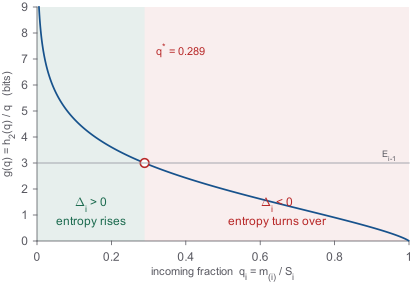
Two identities make the profile cheap to compute and its geometry interpretable. Writing $A_{i} = \sum_{j = 1}^{i} m_{(j)} \log_{2} m_{(j)}$ , the profile has a closed form, and it also satisfies an exact one-step recurrence in the incoming fraction $q_{i} = m_{(i)} / S_{i}$ :

E_{i} = \log_{2} S_{i} - \frac{A_{i}}{S_{i}}, E_{i} = (1 - q_{i}) E_{i - 1} + h_{2} (q_{i}) .

(3)

The recurrence separates the two competing effects exactly. The binary entropy $h_{2} (q_{i})$ is what the incoming object adds by splitting the total mass between itself and everything before it. The factor $(1 - q_{i})$ is what it removes, by contracting every preceding share. Subtracting gives the increment in a form that decides its own sign:

Δ_{i} = E_{i} - E_{i - 1} = q_{i} [g (q_{i}) - E_{i - 1}], g (q) = \frac{h_{2} (q)}{q} .

(4)

Since $g$ is continuous and strictly decreasing from $\infty$ to $0$ on $(0, 1)$ , every prefix with positive entropy has exactly one incoming fraction at which the profile stops rising. Below it the profile rises; above it, it turns over. There is no interval of ambiguity and nothing to calibrate: the crossing is a property of the accumulated measure at that rank.

Figure 2. One crossing, no threshold. The curve is

g (q)

, the horizontal line is the entropy already accumulated. Their single intersection separates an incoming object that adds spread from one that dominates. Drawn for a prefix holding 3 bits, where the crossing sits at

q^{*} = 0.289

; the position moves with the prefix, but there is always exactly one.

A critical relation rather than a chosen number

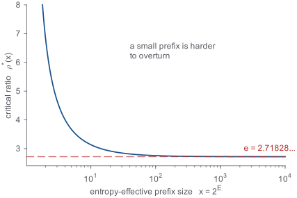
The crossing can be restated in the units a scientist actually thinks in. Let $x = 2^{E_{n}}$ be the entropy-effective size of the prefix, the number of equally weighted objects that would carry the same entropy, and let the incoming value be $ρ$ times the effective mass of one of them. The profile turns over exactly when $ρ$ passes the root of

ρ^{*} \ln ρ^{*} = (x + ρ^{*}) \ln (1 + \frac{ρ^{*}}{x}) .

(5)

The composition of the prefix enters only through $x$ . Whatever the objects are and however their measure is distributed, two prefixes of the same effective size are overturned by the same ratio. That root is always greater than $e$ , decreases in $x$ , and tends to $e$ as the prefix grows.

The critical ratio plotted against the entropy-effective prefix size on a logarithmic axis. It starts above 6 for very small prefixes and decreases monotonically towards a dashed asymptote at e equals 2.718. — **Figure 3. The critical ratio and its universal asymptote.** The ratio at which an incoming value overturns the profile, against the entropy-effective size of what it arrives into. A small prefix is hard to overturn and needs a ratio above 6; by an effective size of 100 the requirement has fallen to 2.76, and the limit is $e$ . The scale separation SPINE responds to is therefore fixed by the construction, not chosen by anyone.

From the profile to strata and scores

A rank is a candidate boundary when the profile has just finished rising, declines strictly at the next admission, and the two measure levels either side of it are genuinely distinct:

𝒞 = {i : E_{i} \geq E_{i - 1}, E_{i} > E_{i + 1}, m_{(i)} < m_{(i + 1)}} .

(6)

The last condition means no boundary can fall inside a block of equal measure values: objects that the measure cannot tell apart are never separated. The retained boundaries cut the sorted order into contiguous strata. Each boundary is then charged with the depth of the descending excursion it starts, and those depths are accumulated into levels:

d_{k} = E_{b_{k}} - min_{b_{k} \leq r \leq b_{k + 1}} E_{r}, ℓ_{k + 1} = \frac{\sum_{j = 1}^{k} d_{j}}{\sum_{j = 1}^{K} d_{j}} .

(7)

Every retained boundary has a strictly positive depth, so the levels increase strictly from $0$ to $1$ . They are relative coordinates on the discovered scale ordering: how much of the total entropy separation has been crossed by the time a stratum is reached. They are not probabilities.

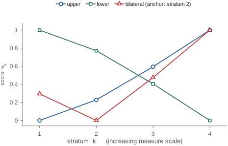
Only now does orientation enter, and it does nothing to the partition. It selects which stratum is the typical one and reads the levels accordingly:

s_{k}^{upper} = ℓ_{k}, s_{k}^{lower} = 1 - ℓ_{k}, s_{k}^{bilateral} = \frac{| ℓ_{k} - ℓ_{k^{*}} |}{max_{j} | ℓ_{j} - ℓ_{k^{*}} |} .

(8)

Each object inherits the score of its stratum. A score of zero is the typical stratum and one is the most separated; nothing further is thresholded.

Scores against stratum index for four strata, under three orientations. Upper rises from 0 to 1 across the strata, lower falls from 1 to 0, and bilateral anchored in stratum two is zero at stratum two and positive on both sides. — **Figure 4. One partition, three readings.** Four scale strata, found once, at separation levels 0, 0.228, 0.595 and 1. Upper orientation calls the largest scale atypical, lower calls the smallest, and bilateral treats a named anchor stratum as typical and scores departure in either direction. The strata, their depths and their levels are identical in all three: orientation is the interpretive layer and never touches the structure.

What the construction guarantees

Every normalized share in equation (1) depends on the measure only through ratios, so multiplying the whole measure by a positive constant leaves the sorted order, the profile, the boundaries, the depths, the levels and every score untouched:

E_{i} (c μ) = E_{i} (μ) for every c > 0 .

(9)

A change of units is therefore not a change of analysis. A nonlinear monotone transformation is: it redistributes the normalized prefix mass and defines a different measure, which is a scientific decision rather than a display one.

The output is deterministic. There is no randomness, no initialisation, no iteration to convergence, and no number of groups to declare. Sorting costs $O (N \log N)$ ; everything after it is linear in $N$ .

When there is nothing to find. A measure with no multiplicative separation produces no transition, and SPINE returns a single unresolved stratum. That is an answer rather than a failure. It says this measure does not separate these objects into scales, which is a statement about the measure that was chosen, not about the cut. The response is a better measure, not a looser setting, because there is nothing to loosen.

The measure is the modelling step

SPINE acts on the values of $μ$ , never on the original representation. Two analyses of the same objects under different measures are therefore two different scientific analyses, and they can disagree about which objects are notable while both being right, because they are answering different questions. Choosing the measure matters more than anything else done with this software, so it has a page of its own.

Choosing a measure →

Reading

Choosing a measure	What a measure has to be, what makes one useful, and how two defensible measures come to disagree. Read before applying SPINE to a problem.
User guide	Worked scenarios in MATLAB: point clouds, networks, spectra, symbolic states, tables and struct arrays.
Function reference	One page per function, with every example executed when the page is built.

The theory and the numerical policy are stated in the paper and its supplementary material; the conformance contract ships with the source as shared fixtures and expected outputs under spec/conformance/. The figures on this page are drawn from the package itself by matlab/doc/buildFigures.m.

Citation

A. R. AlMomani. Scale Partitioning by Incremental Nested Entropy: A Measure-Oriented Theory of Multiscale Structure. Embry-Riddle Aeronautical University, 2026.