Python · chapter 2 of 13

Concepts and conventions

This chapter states the model equations exactly as the code implements them, and the conventions that every function follows.

The regulatory network

A network of n genes is a signed adjacency matrix S of shape (n, n) with entries in {-1, 0, +1}:

• S[i, j] = +1: gene j activates gene i.
• S[i, j] = -1: gene j represses gene i.
• S[i, j] = 0: no direct regulation.

Row i therefore lists the regulators of gene i, and column j lists the targets of gene j. Self-regulation is a nonzero diagonal entry. Any numeric array is accepted; its sign is taken. Gene indices are 0-based; labels ("G1", "G2", ... by default) can be used instead of indices wherever a gene is named.

This orientation, "row = inputs of the node", is shared with the MATLAB toolbox. When you write an edge list, source = j and target = i.

For a three-gene chain A activates B, B represses C, C represses A:

import numpy as np
S3 = np.zeros((3, 3)); S3[1, 0] = 1; S3[2, 1] = -1; S3[0, 2] = -1
m3 = grn.build_model(S3, labels=["A", "B", "C"])
files = grn.export(grn.simulate(m3, duration=1), "abc.csv")
print(open(files[1]).read())          # abc_truth.csv

S3 =
 [[ 0.  0. -1.]
 [ 1.  0.  0.]
 [ 0. -1.  0.]]
source,target,sign
A,B,1
B,C,-1
C,A,-1

One-stage kinetics (default)

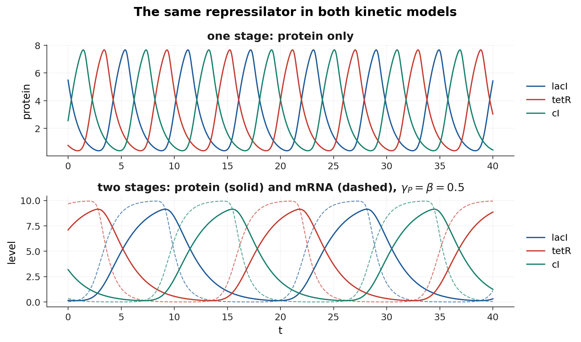
Each gene has one state x_i, read as the level of its product (protein). The dynamics are

dx_i/dt = production_i(x) - gamma_i x_i

where gamma_i is a first-order degradation rate and production_i combines the regulators through Hill functions. For an edge from j to i with threshold K_ij and Hill coefficient h_ij:

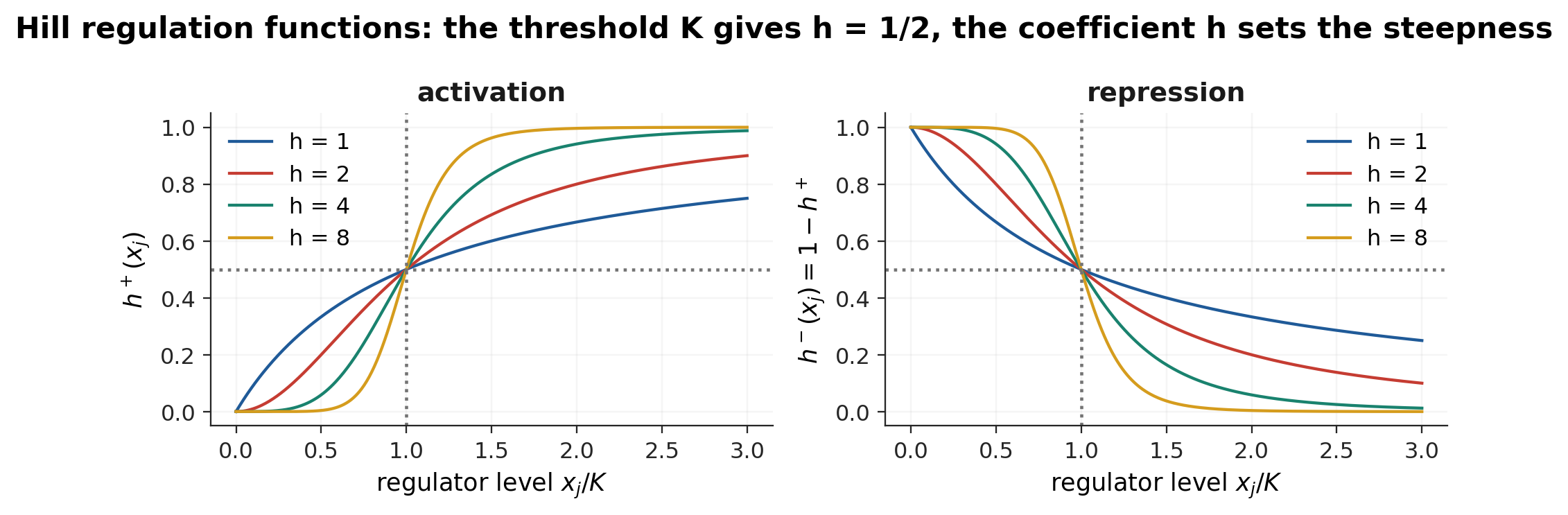
h+(x_j) = x_j^h / (K^h + x_j^h)      activation
h-(x_j) = 1 - h+(x_j)                 repression

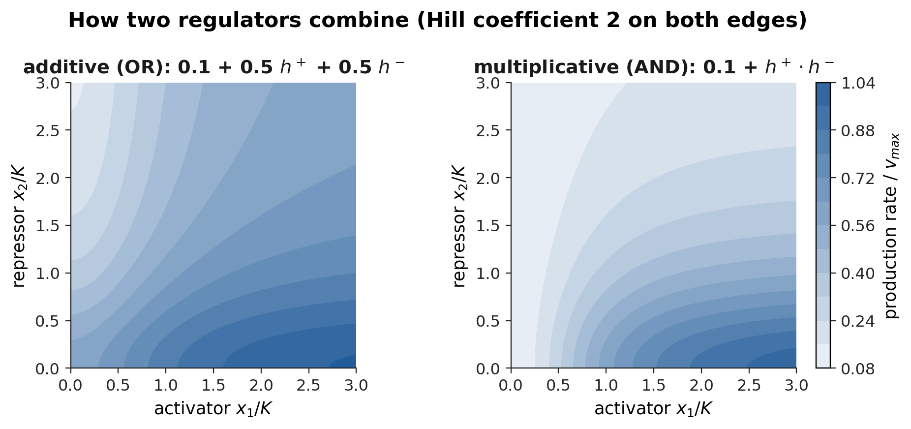
R_ij(x_j) denotes h+ for an activating edge and h- for a repressing edge. Two ways of combining regulators are implemented, selected by logic in grn.build_model:

Genes with no regulators are constitutive: their production is basal_i, which grn.build_model sets equal to vmax_i. Regulated genes get a small leak, basal_i between 0 and 10 % of vmax_i by default.

The Hill coefficient is required to be at least 1 so that the right-hand side is differentiable at zero.

Two-stage kinetics (mRNA and protein)

With stages=2 every gene has an mRNA level m_i and a protein level q_i. Transcription is regulated by the regulators' proteins, translation is linear, and both species degrade:

dm_i/dt = production_i(q) - gamma_i  m_i
dq_i/dt = beta_i m_i     - gammaP_i q_i

The state vector is [m, q], of length 2n, with mRNA first. model.state_labels names the entries (G1_mRNA, ..., G1_protein, ...) and model.state_gene maps each state to its gene. Solutions expose sol.mrna and sol.protein.

At steady state q_i* = (beta_i / gammaP_i) m_i*. By default beta_i = gammaP_i, so protein and mRNA coincide at steady state and the motif presets (whose thresholds K are tuned to the one-stage scale) behave the same way in both models. See Building models for the sampling ranges.

Time and units

Time is dimensionless. Degradation rates default to the range 0.5 to 1.5, so one time unit is roughly one mRNA lifetime. Expression is in arbitrary concentration units set by vmax / gamma, between about 1 and 10 by default. Nothing in the package assumes molecule counts; the chemical Langevin noise model introduces an effective system size through its noise_strength.

Seeds

Every function that draws random numbers has a seed argument, default 0, and creates numpy.random.default_rng(seed) before drawing. seed=None uses NumPy's unseeded entropy. In grn.simulate cell k uses seed + k, and observation noise uses seed + cells; in grn.knockout_screen the seed governs the measurement noise.

The Model object

grn.build_model returns a Model dataclass with these attributes. Parameter arrays are the ground truth for the kinetics; the f, jac, and production callables are rebuilt from them by grn.attach_handles whenever the package changes a parameter.

Models are immutable from the package's point of view: perturb and stimulate return modified copies. If you edit a parameter array by hand, call grn.attach_handles(model) afterwards so the callables see the change. Models pickle cleanly (the callables are rebuilt on load).

What a model looks like at the prompt:

m3

Model(name='grn', n=3, stages=1, logic='additive', edges=3, dim=3)
fields: name, n, S, logic, stages, k, K, hill, basal, gamma, vmax, beta, gammaP, ic, labels, seed, options, perturbation, stimulus, type, dim, hasReg, indegree, outdegree, state_gene, species, state_labels, decay, scale, breaks, f, jac, production

The Solution object

grn.simulate returns a Solution with:

grn.knockout_screen returns a Screen with X ((len(genes) + 1, dim), wild type first), rows, genes, converged, and factor; its type is "screen".

← Getting startedNetworks: motifs and random topologies →