Python · chapter 1 of 13

Getting started

GRNLab generates gene-expression data from gene regulatory networks (GRNs) with Hill-function kinetics. Every dataset it produces comes with the ground truth that generated it: the signed regulatory network, every kinetic parameter, the initial conditions, the seed, and the solver settings. GRNLab is a data generator only. It does not infer, recover, or score networks.

This is the Python guide. The MATLAB toolbox has the same functions, options, conventions, kinetics, and figures; only the naming (snake_case, 0-based indices) and the random-number streams differ.

Installation

pip install grnlab

Requirements: Python 3.9 or newer, NumPy, SciPy, Matplotlib. No other dependencies, no compiled code.

import grnlab as grn

Ten lines to a dataset

import grnlab as grn

grn.catalog()                                          # what is available

S     = grn.random_network(30, topology="scalefree", seed=2)          # ground truth
model = grn.build_model(S, logic="multiplicative", seed=2)            # kinetics
sol   = grn.simulate(model, cells=50, random_ic=True,
                     noise="langevin", noise_strength=0.2,
                     noise_sigma=0.05, seed=2)                        # data

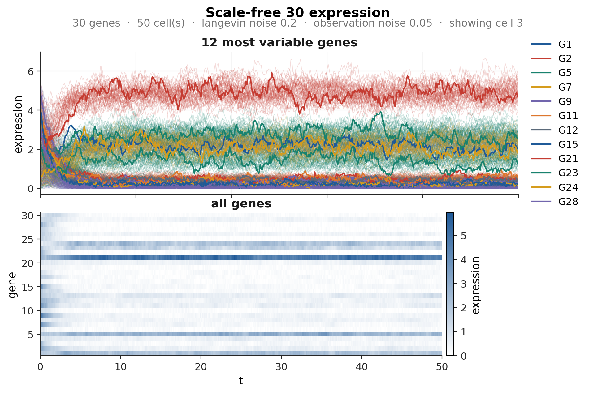
sol.x.shape            # (501, 30, 50): samples x genes x cells
sol.S                  # the signed adjacency that generated the data
grn.plot_network(model)            # arrowheads = activation, bars = repression
grn.plot_expression(sol, cell=2)
grn.export(sol, "grn30.csv")       # + grn30_truth.csv, grn30_adjacency.csv

Output

Regulatory motifs (grnlab.motif / grnlab.build_model):
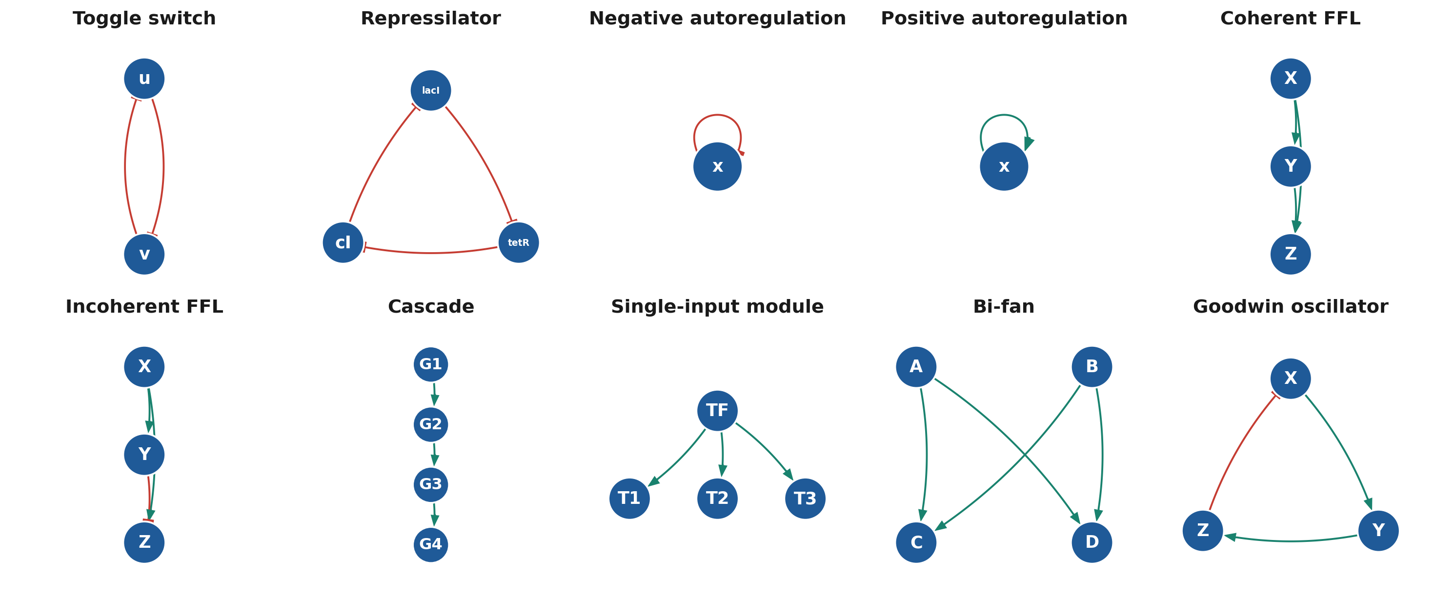
    toggle           2   Toggle switch: mutual repression, bistable for cooperative binding
    repressilator    3   Repressilator: three-gene ring of repressors, limit-cycle oscillator
    nar              1   Negative autoregulation: fast, robust response
    par              1   Positive autoregulation: slow, possibly bistable
    ffl_coherent     3   Coherent type-1 feed-forward loop: sign-sensitive delay
    ffl_incoherent   3   Incoherent type-1 feed-forward loop: pulse generator
    cascade          4   Linear activation cascade of 4 genes
    sim              4   Single-input module: one TF driving 3 targets
    bifan            4   Bi-fan: two TFs jointly regulating two targets
    goodwin          3   Goodwin oscillator: activation chain closed by repression
Random topologies (grnlab.random_network topology option):
    erdosrenyi   independent edges, Poisson in-degree
    scalefree    preferential attachment on regulators (hub TFs)
    smallworld   directed ring lattice with random rewiring
    modular      dense modules with sparse inter-module edges

Output

sol.x.shape = (501, 30, 50)
sol.S[:6, :6] =
 [[ 0. -1. -1.  0.  0.  0.]
 [-1.  0.  1.  0.  0.  0.]
 [-1.  1.  0.  0.  0.  0.]
 [ 0. -1.  1.  0.  0.  0.]
 [ 1. -1.  0.  0.  0.  0.]
 [ 0. -1.  1.  0.  0.  0.]]
sol.labels[:6] = ('G1', 'G2', 'G3', 'G4', 'G5', 'G6')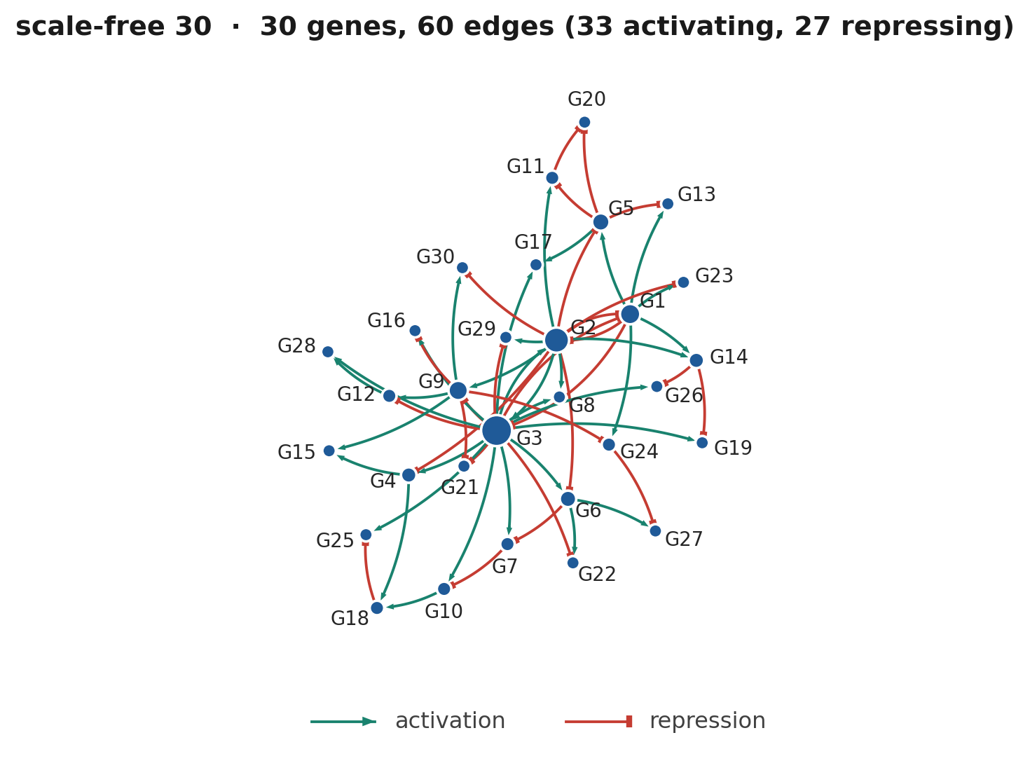

The ground truth of the example: 30 genes, 60 edges. Arrowheads mark activation, bars mark repression, and node size grows with the number of targets, so the hub regulators stand out.

Cell 3 of the 50 cells. Top: the twelve most variable genes, with the other 49 cells drawn faintly behind. Bottom: all 30 genes as a genes-by-time heat map. Genes without regulators sit at their constitutive level; most others are held down by the repressor-heavy hubs.

Output

grn30.csv
grn30_truth.csv
grn30_adjacency.csv

The three objects you will handle

Object	Made by	What it holds
Adjacency `S`	`grn.random_network`, `grn.motif`, or your own array	The signed network: `S[i, j] = +1` if gene j activates gene i, `-1` if it represses it, `0` otherwise
Model	`grn.build_model`	`S` plus every kinetic parameter, the initial condition, and callables for the right-hand side and Jacobian
Solution / Screen	`grn.simulate`, `grn.knockout_screen`	The data, the time grid, the model that produced it, and the options used

Everything downstream (perturbations, stimuli, steady states, plots, export) takes a model or a solution and never loses the ground truth.

Motifs by name

Ten classic motifs are registered with parameter presets that reproduce their textbook behaviour. A motif name can be used wherever a model is expected:

sol = grn.simulate("repressilator")             # oscillates
model = grn.build_model("toggle")               # bistable
hi = grn.steady_state(model, initial_condition=[5, 0])
lo = grn.steady_state(model, initial_condition=[0, 5])
grn.plot_motifs()                               # gallery of all ten

Output

hi = [4.7913 0.2087]
lo = [0.2087 4.7913]

The ten registered motifs. Feed-forward motifs are laid out with regulators above their targets; autoregulation is a loop.

Reproducibility

Every random choice is driven by a seed argument that defaults to 0. Network topology, parameter sampling, random initial conditions, process noise, and observation noise are all seeded, and cell k of a multi-cell simulation uses seed + k. Rerunning the same call gives bit-identical data. seed=None leaves NumPy's generator unseeded. The solution records the seed and every option, so sol.options and sol.model are a complete recipe.

Where next

Concepts and conventions: the equations, the orientation of S, and the attributes of a model.
Simulating expression data: solvers, cells, noise, and the solution object.
Recipes: complete workflows for benchmark datasets, dose-response experiments, and DREAM-style packages.
Function reference: every function and argument on one page.

Concepts and conventions →