Python · chapter 3 of 13

Networks: motifs and random topologies

A network is just a signed adjacency array, so you can build one by hand, take a registered motif, or draw one at random.

By hand

import numpy as np
S = np.zeros((3, 3))
S[1, 0] = 1       # G1 activates G2
S[2, 1] = -1      # G2 represses G3
model = grn.build_model(S, labels=["A", "B", "C"])

Registered motifs

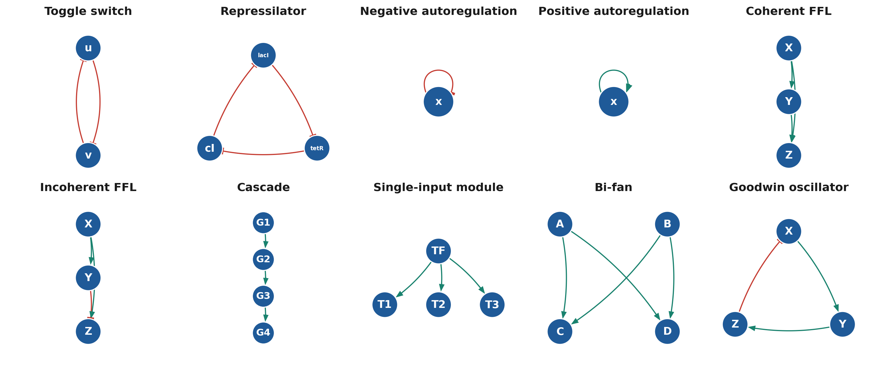
grn.motif(name) returns a Motif with attributes name, S, labels, description, and preset, the parameter overrides that grn.build_model applies automatically when it is given the motif name. grn.catalog() lists them.

Name	Genes	Structure	Preset behaviour
`"toggle"`	2	u and v repress each other	Bistable: Hill 2, alpha = 5
`"repressilator"`	3	lacI -\	tetR -\	cI -\	lacI	Limit-cycle oscillator: Hill 4, alpha = 10
`"nar"`	1	x represses itself	Fast, robust response
`"par"`	1	x activates itself	Slow response, possibly bistable
`"ffl_coherent"`	3	X -> Y, X -> Z, Y -> Z	Sign-sensitive delay (AND gate with multiplicative logic)
`"ffl_incoherent"`	3	X -> Y, X -> Z, Y -\	Z	Pulse generator
`"cascade"`	`size` (4)	G1 -> G2 -> ...	Linear activation chain
`"sim"`	`size` (4)	TF -> T1, T2, ...	Single-input module
`"bifan"`	4	A, B -> C, D	Two regulators, two targets
`"goodwin"`	3	X -> Y -> Z -\	X	Oscillator: Hill 8, alpha = 10

m = grn.motif("cascade", size=6)
model = grn.build_model(m)                         # labels kept, no preset
model = grn.build_model("cascade")                 # with the preset, size 4

The presets set k, vmax, K, hill, gamma, and basal where the textbook behaviour depends on them. You can override any of them through params.

grn.plot_motifs(): every registered motif in pathway notation.

Random topologies

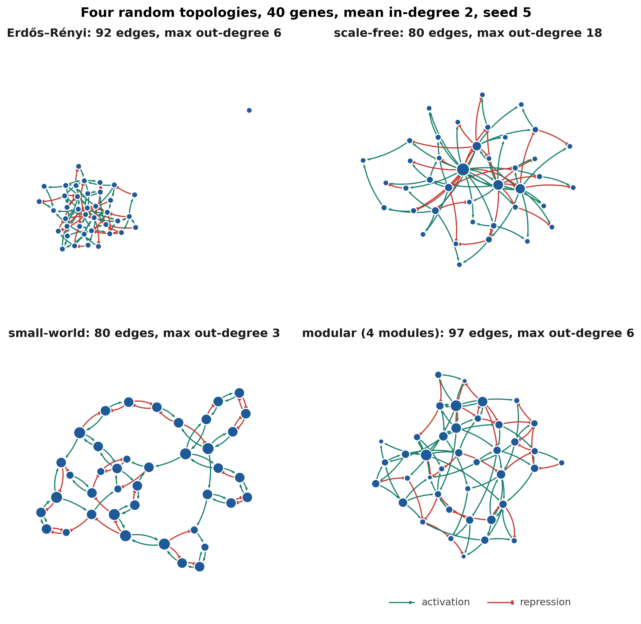
S = grn.random_network(n, ...) draws a signed adjacency with n genes; S, info = grn.random_network(n, ..., info=True) also returns generator details.

Argument	Default	Meaning
`topology`	`"erdosrenyi"`	`"erdosrenyi"`, `"scalefree"`, `"smallworld"`, or `"modular"`
`mean_degree`	2	Expected number of regulators per gene
`fraction_repressors`	0.4	Probability that an edge represses
`self_regulation`	0	Probability that a gene regulates itself
`modules`, `within_fraction`	4, 0.8	Modular topology: number of modules and fraction of edges inside modules
`rewire`	0.1	Small-world topology: rewiring probability
`seed`	0	Seed
`info`	False	Also return `dict(topology, modules, mean_degree)`

How each topology is drawn:

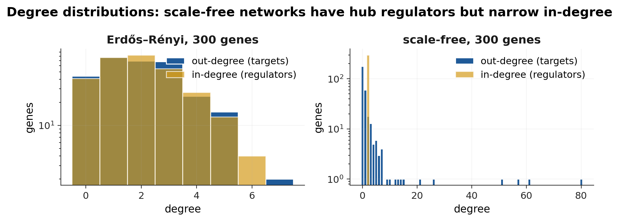
Erdős–Rényi. Every ordered pair (i, j), i ≠ j, gets an edge independently with probability mean_degree / (n - 1). In-degrees are Poisson-like.
Scale-free. Genes are added one at a time. Each new gene picks round(mean_degree) regulators among the existing genes with probability proportional to their out-degree + 1. Early genes become hub transcription factors with many targets; in-degree stays narrow, which matches real regulatory networks better than an undirected Barabási–Albert graph.
Small-world. Each gene is regulated by its round(mean_degree) nearest neighbours on a ring; each edge is then rewired to a random regulator with probability rewire.
Modular. A stochastic block model with modules equal blocks; edge probabilities are chosen so that a fraction within_fraction of the expected mean_degree * n edges fall inside modules. info["modules"] returns the block of every gene.

After the topology, each edge is made repressing with probability fraction_repressors, and each gene gets a self-loop with probability self_regulation (sign drawn the same way). info["mean_degree"] reports the realised mean in-degree.

The four topologies at 40 genes and mean in-degree 2. Scale-free networks concentrate outgoing edges on a few hub regulators; modular networks show dense blocks with sparse links between them.

Out-degree (targets per gene) and in-degree (regulators per gene) at 300 genes. The scale-free generator produces hubs with tens of targets while keeping the in-degree narrow, which is how real transcription networks look.

S, info = grn.random_network(60, topology="modular", modules=3,
                             mean_degree=2.5, seed=4, info=True)
info
np.count_nonzero(S), np.count_nonzero(S, axis=1)

Output

info = {'topology': 'modular', 'modules': 'array(60,)', 'mean_degree': np.float64(2.5166666666666666)}
edges = 151
in-degree = [1 3 2 2 3 3 3 3 2 4 4 3 1 1 2 3 3 4 0 4 1 5 4 3 1 9 3 1 1 5 5 2 2 2 0 1 2 3 1 4 4 2 1 3 0 1 4 4 0
 2 0 3 1 4 3 1 5 1 2 4]

Checking a network

A few one-liners that are useful before building a model:

np.count_nonzero(S)                    # number of edges
np.count_nonzero(S, axis=1)            # in-degree (regulators per gene)
np.count_nonzero(S, axis=0)            # out-degree (targets per gene)
np.nonzero(~S.any(axis=1))[0]          # source genes: constitutive, no regulators
np.count_nonzero(np.diag(S))           # self-regulating genes

← Concepts and conventions Building models →