MATLAB · chapter 8 of 13
Figures
Every plotting function returns a figure handle and follows one house style (palette, typography, tick and grid styling). Pair them with grn.exportFigure for publication output.
Networks: grn.plotNetwork
fig = grn.plotNetwork(model) accepts a model, a solution, a screen (anything with a field S), or a signed adjacency. It draws the network in pathway notation:
- Activation ends in a filled arrowhead, repression in a bar.
- Autoregulation is a loop bulging away from the network's centre.
- Reciprocal edges curve apart so both directions stay visible.
- Node size grows with the number of targets, so hub regulators stand out.
- Labels sit inside the nodes up to 12 genes and beside them beyond that, placed in the emptiest direction.
| Option | Default | Meaning |
|---|---|---|
Layout | "auto" | "circle" (up to 12 genes), "force" (beyond), or "layered" with regulators above targets |
Labels | true up to 60 genes | Show gene labels |
Curvature | 0.12 | Edge bend as a fraction of edge length (reciprocal edges bend at least 0.22) |
Axes | new figure | Draw into an existing axes, for your own tiled layouts |
Title, Legend | true | Show the title line and the activation/repression key |
Seed | 1 | Seed for the force layout |
fig = grn.plotNetwork(model, Layout = "layered");
grn.exportFigure(fig, "network.pdf");           % vector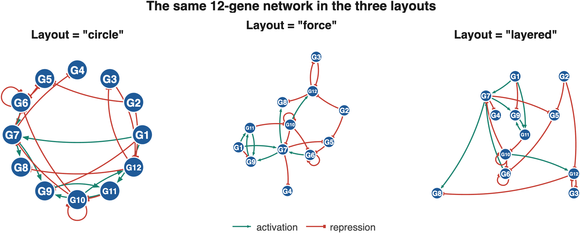
Motif gallery: grn.plotMotifs
grn.plotMotifs() draws all ten registered motifs; grn.plotMotifs(["toggle", "repressilator"]) a subset. Options Columns (5) and Size (4, for cascade and sim).
Expression data: grn.plotExpression
fig = grn.plotExpression(sol, ...) shows a solution as line traces (all genes up to MaxLines, otherwise the most variable ones) over a genes-by-time heat map. When the solution has several cells, the chosen cell is drawn in full and the others as faint traces behind it. When a stimulus was applied, a top panel shows the input.
| Option | Default | Meaning |
|---|---|---|
Cell | 1 | Which cell to draw in full |
MaxLines | 12 | Maximum number of traces |
Overlay | true | Draw the other cells faintly (up to 50 cells) |
Species | "protein" | "protein" or "mrna" for two-stage models |
Export: grn.exportFigure
grn.exportFigure(fig, filename) applies the house style and writes the file. .png, .jpg, .tif are rasterised at Resolution dpi (default 300); .pdf and .eps are true vector graphics. Style = false skips the restyling.
grn.exportFigure(fig, "figure3.png", Resolution = 600);
grn.exportFigure(fig, "figure3.pdf");
Headless sessions (matlab -batch) work; the style forces a light theme so exports do not inherit the dark desktop theme of recent releases.
Building your own figure
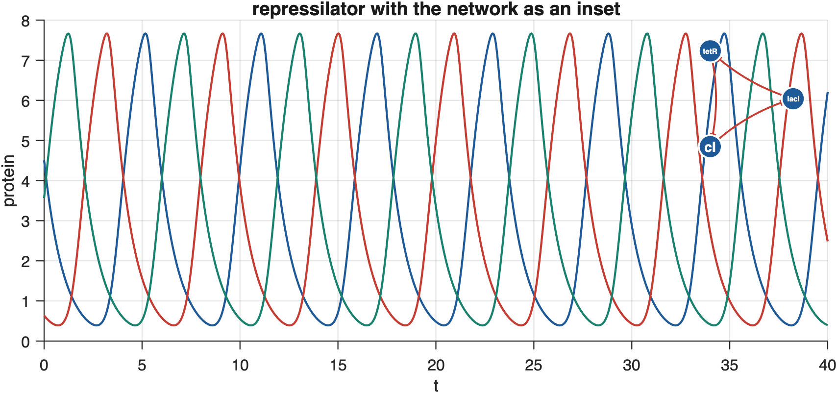
The style constants are available for custom plots:
st = grn.internal.style();     % st.colors (7 x 3), st.gray, st.fontName, st.lineWidth, ...
fig = figure(Color = "w");
ax = axes(fig); hold(ax, "on");
plot(ax, sol.t, sol.x(:, 1), Color = st.colors(1, :), LineWidth = st.lineWidth);
grn.plotNetwork(model, Axes = axes(fig, Position = [0.7, 0.6, 0.28, 0.35]), Title = false, Legend = false);
grn.exportFigure(fig, "custom.pdf");
grn.internal.applyStyle(fig) restyles any figure in place.