MATLAB · chapter 6 of 13

Perturbations, steady states, and knockout screens

Genetic perturbations

grn.perturb scales the production of chosen genes: the basal rate, the maximal rate vmax, every incoming weight k(i, :), and the gene's entries in model.ic. Genes may be given as indices or labels.

Option	Factor	Effect
`Knockout`	0	No production; the gene decays to zero and stays there
`Knockdown`	`KnockdownFactor` (0.5)	Reduced production
`Overexpress`	`OverexpressFactor` (2)	Increased production

ko = grn.perturb(model, Knockout = [2, 5]);
kd = grn.perturb(model, Knockdown = "G7", KnockdownFactor = 0.25);
sol = grn.simulate(model, Knockout = 4, Overexpress = "G7");   % same options

The perturbation is recorded in model.perturbation.gene and .factor. Perturbations accumulate if you call grn.perturb repeatedly; grn.simulate, grn.steadyState, and grn.knockoutScreen always start from the model you pass them.

Knockouts act on production, not on the network: the ground truth S is unchanged, which is what a benchmark needs. In two-stage models the transcription of the gene is scaled, so both its mRNA and its protein go to zero.

model = grn.buildModel("cascade", Seed = 1);
wt = grn.simulate(model, InitialCondition = zeros(4, 1), Duration = 20);
ko = grn.simulate(model, InitialCondition = zeros(4, 1), Duration = 20, Knockout = "G2");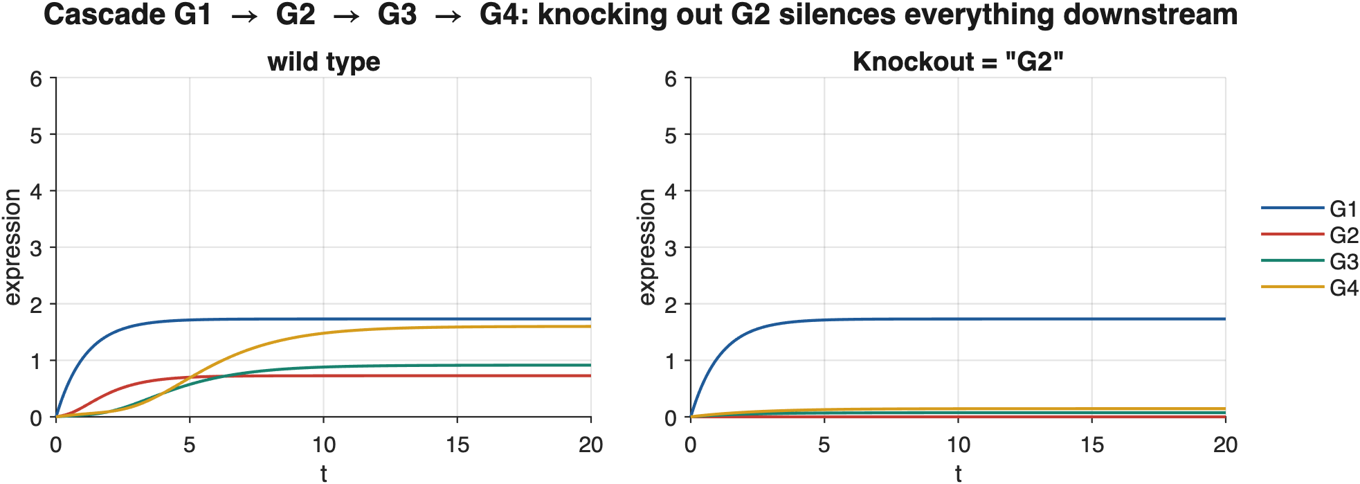

A four-gene activation cascade switched on from zero, wild type and with G2 knocked out. G2 stays at zero and everything downstream is silenced, while the constitutive G1 is unaffected.

Steady states

[xss, info] = grn.steadyState(model, ...) finds a fixed point in two phases: it integrates with ode15s (using the analytic Jacobian) in windows of 20 / min(decay) until the relative residual norm(f) / (1 + norm(x)) drops below Tol (1e-8) or MaxTime (2000) is exceeded, then polishes with Newton steps until the residual is at machine precision.

Output	Meaning
`xss`	The fixed point, `dim x 1`; if the model never settles, the time average over the last window
`info.converged`	Whether a fixed point was reached
`info.stable`	All Jacobian eigenvalues at `xss` have negative real part
`info.residual`, `info.time`	Final `norm(f)` and integration time used

Options: InitialCondition (the starting point, which selects the attractor of a multistable model), MaxTime, Tol, the perturbation options, and Stimulus with Time (stimuli are frozen at their value at Time, default 0).

model = grn.buildModel("toggle");
[hi, info] = grn.steadyState(model, InitialCondition = [5; 0]);   % u high
lo = grn.steadyState(model, InitialCondition = [0; 5]);           % v high
[~, info] = grn.steadyState("repressilator");   % info.converged = false

Output

hi =

    4.7913
    0.2087

info = 

  <a href="matlab:helpPopup('struct')" style="font-weight:bold">struct</a> with fields:

    converged: 1
     residual: 1.9429e-16
         time: 40
       stable: 1
        time0: 0
        model: [1×1 struct]

Knockout screens

screen = grn.knockoutScreen(model, ...) produces the steady-state dataset used by the DREAM challenges: the wild type followed by one row per single-gene perturbation.

Option	Default	Meaning
`Type`	`"knockout"`	`"knockout"`, `"knockdown"`, or `"overexpress"`
`Factor`	0, 0.5, or 2 by type	Production scaling
`Genes`	all	Which genes to perturb, indices or labels
`NoiseSigma`	0	Gaussian measurement noise on `screen.X` (clean copy in `screen.xClean`)
`Seed`	0	Seed for the measurement noise
`Stimulus`, `Time`		Inputs held at their value at `Time`
`MaxTime`, `Tol`		As in `grn.steadyState`

Each perturbed steady state is computed from the wild-type steady state with the perturbed gene's states scaled by the factor, which keeps the screen on the same attractor branch as the wild type in multistable networks.

Output	Meaning
`X`	`(numel(Genes) + 1) x dim`; row 1 wild type, row i + 1 the perturbation of `Genes(i)`
`rows`	Row names: `"wildtype"` then the gene labels
`converged`	Logical per row
`mrna`, `protein`	The two halves of `X` for two-stage models
`S`, `model`, `labels`, `stateLabels`, `options`	Ground truth and settings

ko = grn.knockoutScreen(model, NoiseSigma = 0.05);
kd = grn.knockoutScreen(model, Type = "knockdown", Genes = ["G1", "G4"]);
wt = ko.X(1, :);
lfc = log2((ko.X(2:end, :) + 1e-3) ./ (wt + 1e-3));   % log fold change per knockout
grn.export(ko, "screen.csv");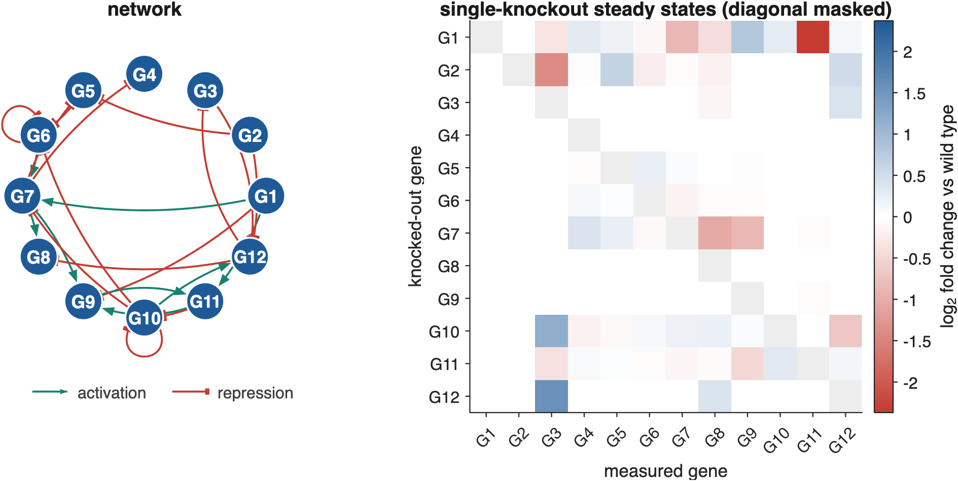

A 12-gene network with two autoregulating genes beside its single-knockout screen, shown as log2 fold change against wild type with the knocked-out gene itself masked. Knocking out a repressor raises its targets (blue); knocking out an activator lowers them (red). Every off-diagonal effect has the sign the network predicts.

The first rows and columns of the screen:

array2table(round(ko.X(1:5, 1:6), 3), VariableNames = ko.labels(1:6), RowNames = ko.rows(1:5))

Output

                 <strong>G1</strong>       <strong>G2</strong>      <strong>G3</strong>       <strong>G4</strong>       <strong>G5</strong>       <strong>G6</strong>  
                <strong>_____</strong>    <strong>____</strong>    <strong>_____</strong>    <strong>_____</strong>    <strong>_____</strong>    <strong>_____</strong>

    <strong>wildtype</strong>    3.423    1.75    2.358    3.002    0.432    1.586
    <strong>G1      </strong>        0    1.75    1.876    3.722    0.493    1.487
    <strong>G2      </strong>    3.423       0    0.888    3.064    0.664    1.368
    <strong>G3      </strong>    3.423    1.75        0    3.002    0.432    1.586
    <strong>G4      </strong>    3.423    1.75    2.358        0    0.432    1.586

A useful sanity check on any screen: knocking out an activator lowers its targets and knocking out a repressor raises them. The audit in Accuracy and validation verifies this on a random network.

Double perturbations and dose series

Combine the options directly:

sol = grn.simulate(model, Knockout = 1, Knockdown = 3);
for f = [0, 0.25, 0.5, 0.75, 1]
    x(:, end + 1) = grn.steadyState(model, Knockdown = 2, KnockdownFactor = f);
end

← Simulating expression data Time-varying stimuli →