MATLAB · chapter 10 of 13

Recipes

Complete, copy-and-run workflows. Each one ends with data and its ground truth on disk.

1. A benchmark time-series dataset

Fifty cells of a 30-gene scale-free network with intrinsic and measurement noise.

S     = grn.randomNetwork(30, Topology = "scalefree", MeanDegree = 2, ...
            FractionRepressors = 0.4, Seed = 2);
model = grn.buildModel(S, Logic = "multiplicative", Seed = 2, Name = "sf30");
sol   = grn.simulate(model, Cells = 50, RandomIC = true, Duration = 20, ...
            SampleDt = 0.25, Noise = "langevin", NoiseStrength = 0.2, ...
            NoiseSigma = 0.05, Seed = 2);
grn.export(sol, "sf30_timeseries.csv");
grn.export(sol, "sf30_timeseries.mat");
fig = grn.plotNetwork(model);        grn.exportFigure(fig, "sf30_network.pdf");
fig = grn.plotExpression(sol, Cell = 1); grn.exportFigure(fig, "sf30_expression.png");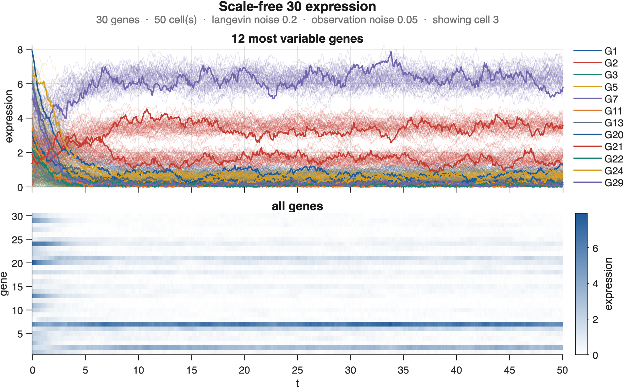

2. A DREAM-style package: knockouts, knockdowns, and wild-type time series

model = grn.buildModel(grn.randomNetwork(10, Seed = 3), Seed = 3, Name = "net10");
ko = grn.knockoutScreen(model, NoiseSigma = 0.02, Seed = 3);
kd = grn.knockoutScreen(model, Type = "knockdown", NoiseSigma = 0.02, Seed = 4);
ts = grn.simulate(model, Cells = 10, RandomIC = true, Duration = 20, ...
        NoiseSigma = 0.02, Seed = 5);
grn.export(ko, "net10_knockouts.csv");
grn.export(kd, "net10_knockdowns.csv");
grn.export(ts, "net10_timeseries.csv");
all(ko.converged) && all(kd.converged)     % check before shipping

3. A dose-response experiment

Steady-state expression of every gene as a source gene is driven from 0 to 3 times its normal rate.

model = grn.buildModel(grn.motif("sim", Size = 5), Seed = 1);   % keeps labels TF, T1..T4
doses = linspace(0, 3, 13);
X = zeros(numel(doses), model.dim);
for d = 1:numel(doses)
    s = grn.stimulus("TF", "step", Baseline = doses(d), Amplitude = doses(d));
    X(d, :) = grn.steadyState(model, Stimulus = s).';
end
plot(doses, X(:, 2:end)); xlabel("input to TF"); ylabel("target expression")

A ramp gives the same information dynamically:

ramp = grn.stimulus("TF", "ramp", Baseline = 0, Amplitude = 3, Start = 0, Stop = 60);
sol = grn.simulate(model, Stimulus = ramp, Duration = 80);
grn.plotExpression(sol);

4. Single-cell-like snapshots

Many cells, one sample each at a random time after a stimulus.

model = grn.buildModel(grn.randomNetwork(20, Seed = 6), Stages = 2, Seed = 6);
on = grn.stimulus(1, "step", Amplitude = 4, Start = 0);
sol = grn.simulate(model, Stimulus = on, Cells = 200, RandomIC = true, ...
    Noise = "langevin", NoiseStrength = 0.3, Duration = 10, SampleDt = 0.1, Seed = 6);
rng(6);
tIdx = randi(numel(sol.t), sol.cells, 1);               % one time per cell
cellsX = zeros(sol.cells, sol.n);
for c = 1:sol.cells
    cellsX(c, :) = sol.mrna(tIdx(c), :, c);              % mRNA, like a scRNA-seq readout
end
pseudotime = sol.t(tIdx);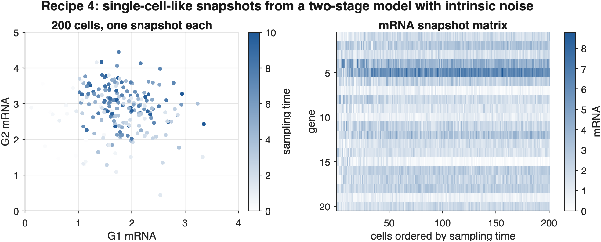

5. Comparing motif variants

Coherent and incoherent feed-forward loops under the same step input.

on = grn.stimulus("X", "step", Baseline = 0, Amplitude = 1, Start = 2);
for name = ["ffl_coherent", "ffl_incoherent"]
    model = grn.buildModel(name, Logic = "multiplicative", Seed = 1, ...
        Params = struct("gamma", [5; 1; 3], "vmax", 5, "basal", [5; 0; 0]));
    sol = grn.simulate(model, Stimulus = on, InitialCondition = zeros(3, 1), Duration = 20);
    fig = grn.plotExpression(sol); grn.exportFigure(fig, name + ".pdf");
end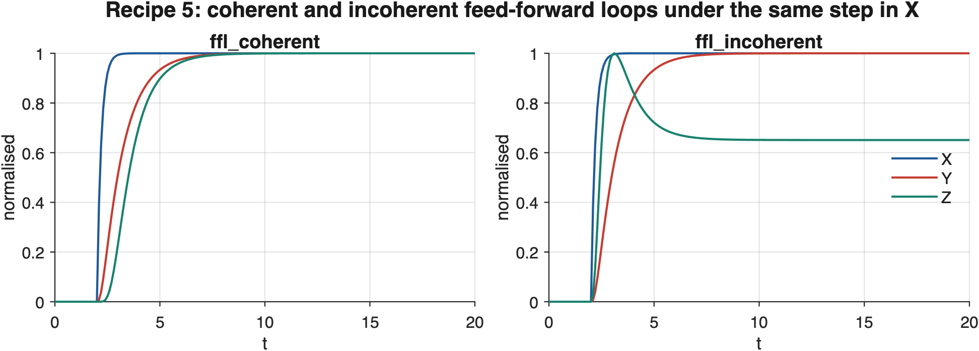

6. A population of related networks

Ten networks that share a topology but differ in kinetics.

S = grn.randomNetwork(15, Seed = 1);
for k = 1:10
    model = grn.buildModel(S, Seed = k, Name = "net15_" + k);
    sol = grn.simulate(model, Cells = 5, RandomIC = true, Seed = k);
    grn.export(sol, sprintf("net15_%02d.mat", k));
end

7. Sweeping a parameter of a motif

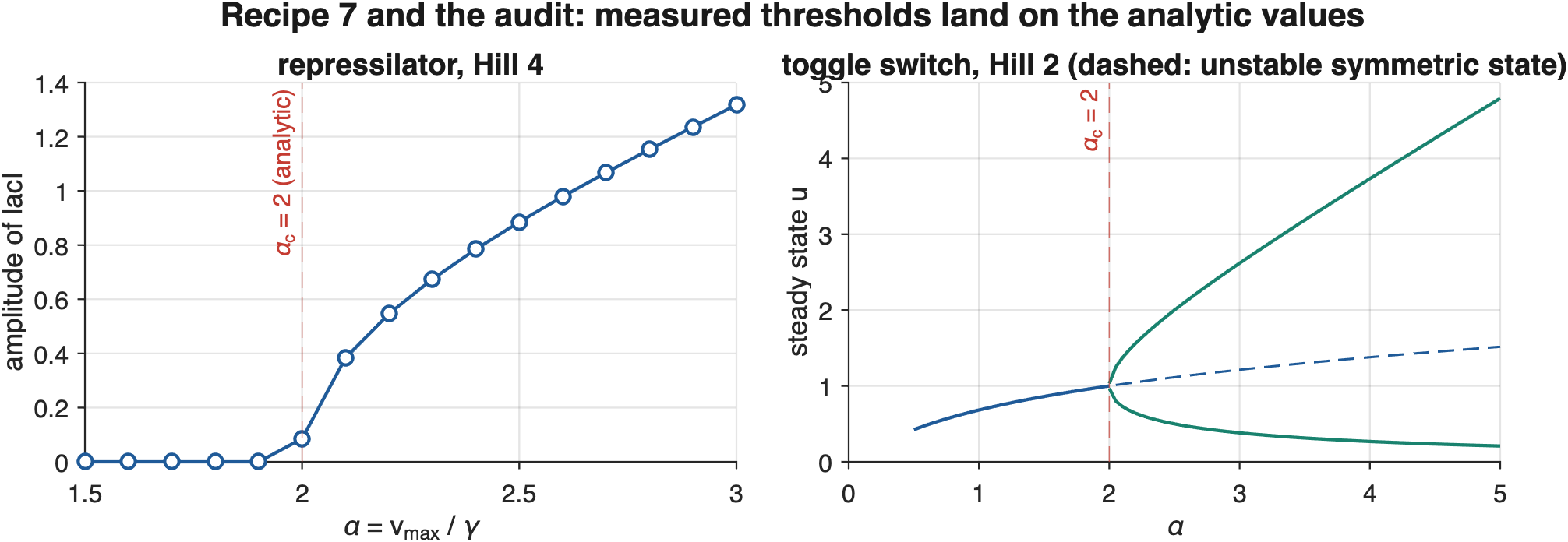
Where does the repressilator start to oscillate? (The analytic answer for Hill 4 is alpha = 2.)

alphas = 1.5:0.1:3;
amp = zeros(size(alphas));
for a = 1:numel(alphas)
    m = grn.buildModel("repressilator", Params = struct("k", alphas(a), "vmax", alphas(a)));
    sol = grn.simulate(m, Duration = 100, Transient = 300);
    amp(a) = max(sol.x(:, 1)) - min(sol.x(:, 1));
end
plot(alphas, amp, "o-"); xlabel("\alpha"); ylabel("amplitude")

← Exporting data and reproducing itAccuracy and validation →