MATLAB · chapter 7 of 13

Time-varying stimuli

Real experiments switch genes on, wash inducers out, ramp a dose, or drive a circuit periodically. grn.stimulus describes such an input and grn.simulate (or grn.stimulate, grn.steadyState, grn.knockoutScreen) applies it.

How a stimulus enters the model

A stimulus acts on the production (transcription) rate of one or more genes through a waveform u(t):

`Mode`	Production of gene i	Interpretation
`"scale"` (default)	`u(t) * production_i(x)`	An inducible promoter: `u = 0` silences the gene, `u = 1` is the unstimulated rate, `u = 3` triples it
`"add"`	`production_i(x) + u(t)`	An external source of transcript in production units

Scale stimuli on the same gene multiply, add stimuli sum. Regulation by the network still applies: a stimulated gene with repressors bound still produces little.

Waveforms

s = grn.stimulus(gene, type, ...) where gene is an index, a label, or a list of either.

`type`	`u(t)`	Options
`"step"`	`Amplitude` for `Start <= t < Stop`, `Baseline` elsewhere	`Start` (0), `Stop` (Inf), `Rise` (0)
`"ramp"`	`Baseline` before `Start`, linear to `Amplitude` at `Stop`, `Amplitude` after	`Start`, `Stop` (required)
`"sine"`	`Baseline + (Amplitude - Baseline) (1 - cos(2 pi (t - Start) / Period)) / 2` for `Start <= t < Stop`	`Period` (10), `Start`, `Stop`
`"custom"`	`Function(t)`	`Function` (required), `Breaks`

Defaults: Baseline = 1 and Amplitude = 2 for scale mode, Baseline = 0 and Amplitude = 1 for add mode. A step with a finite Stop is a pulse. Rise > 0 replaces the jumps of a step by logistic ramps with roughly that 10–90 % rise time, for experiments where the inducer diffuses in.

on    = grn.stimulus("X", "step", Baseline = 0, Amplitude = 1, Start = 5);
pulse = grn.stimulus(1, "step", Amplitude = 3, Start = 5, Stop = 10);
dose  = grn.stimulus(1, "ramp", Baseline = 0, Amplitude = 3, Start = 0, Stop = 40);
drive = grn.stimulus("G2", "sine", Amplitude = 3, Period = 12);
custom = grn.stimulus(1, "custom", Function = @(t) 1 + 0.5 * (t > 3) + 0.5 * (t > 6), Breaks = [3, 6]);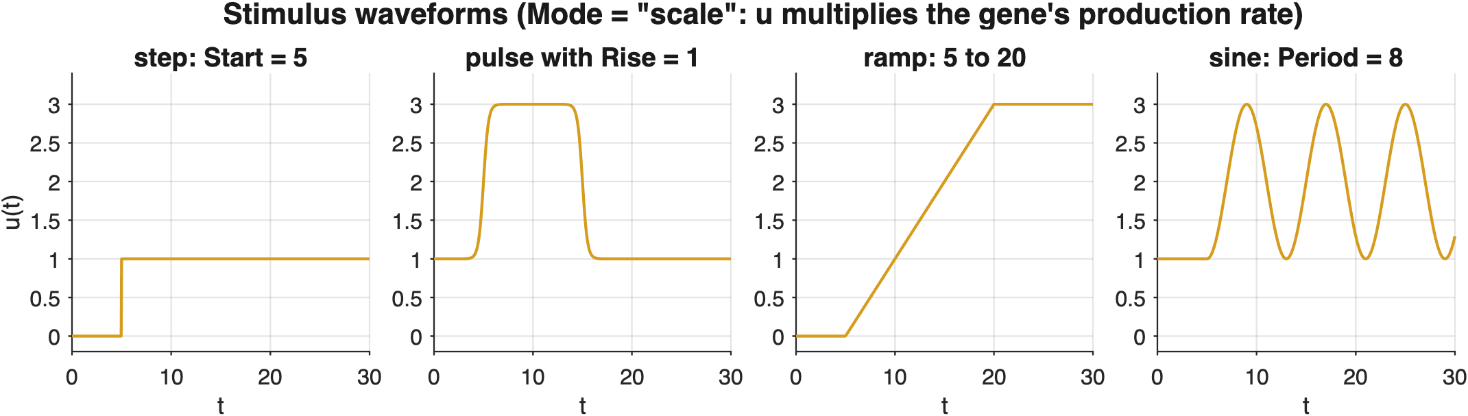

The built-in waveforms. A step with a finite Stop is a pulse, and Rise turns its edges into logistic ramps.

Timing and the solver

Stimulus times are on the clock of the recorded solution: t = 0 is the first recorded sample and a Transient runs at negative times. Every step edge, ramp corner, sine window edge, and custom Breaks time is passed to the ODE integrator, which restarts there. A gene switched on at t = 4 is therefore exactly zero before t = 4, not leaked across a solver step. The Euler–Maruyama integrator evaluates the stimulus at every step.

Applying stimuli

sol = grn.simulate(model, Stimulus = on, Duration = 30);          % one
sol = grn.simulate(model, Stimulus = [on, drive], Duration = 60);  % several
model2 = grn.stimulate(model, pulse);      % attach permanently; model2.f(t, x) includes it
model2 = grn.stimulate(model2, []);        % remove all stimuli

The realised input is recorded in sol.u (the multiplicative factor, samples x n, all ones without stimuli) and sol.uAdd (the additive term). grn.plotExpression adds a panel showing the input when the solution carries a stimulus.

[sol.t(48:53), sol.u(48:53, :)]      % the input around the edge at t = 5

Output

ans =

    4.7000         0    1.0000    1.0000
    4.8000         0    1.0000    1.0000
    4.9000         0    1.0000    1.0000
    5.0000    1.0000    1.0000    1.0000
    5.1000    1.0000    1.0000    1.0000
    5.2000    1.0000    1.0000    1.0000

Steady states under a stimulus

Steady states need an autonomous system. grn.steadyState and grn.knockoutScreen freeze the stimulus at its value at Time (default 0):

off = grn.steadyState(model, Stimulus = on, Time = 0);    % before the step
xon = grn.steadyState(model, Stimulus = on, Time = 10);   % after it
ko  = grn.knockoutScreen(model, Stimulus = on, Time = 10);

This is how to build dose-response steady-state data: a step of each amplitude, Time anywhere after Start.

model = grn.buildModel(grn.motif("sim", Size = 5), Seed = 1);
doses = linspace(0, 3, 13);
for d = 1:numel(doses)
    s = grn.stimulus("TF", "step", Baseline = doses(d), Amplitude = doses(d));
    X(d, :) = grn.steadyState(model, Stimulus = s).';
end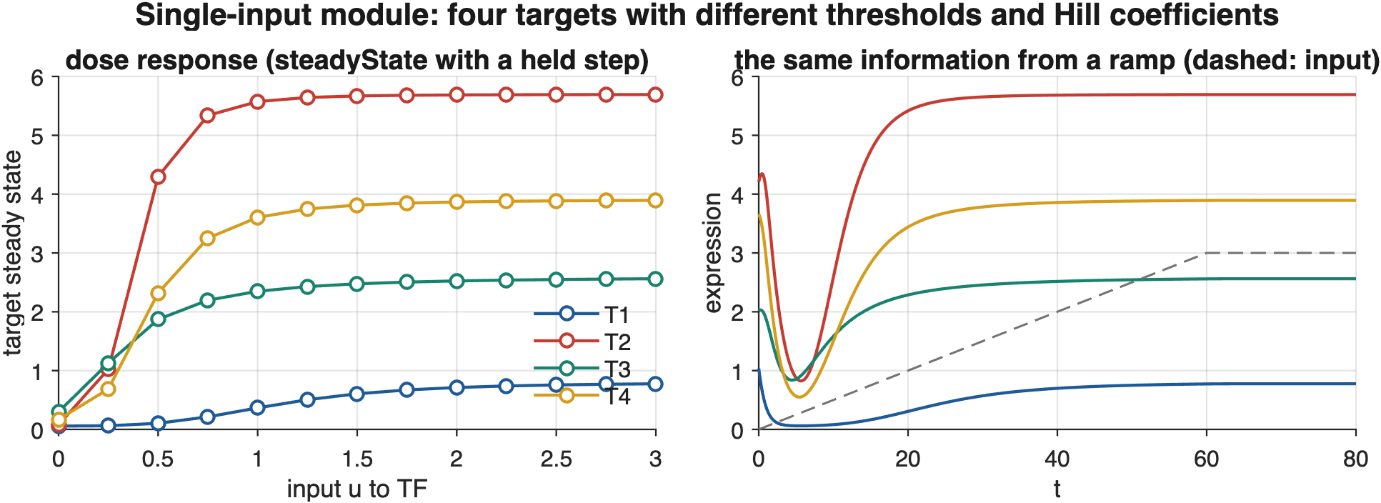

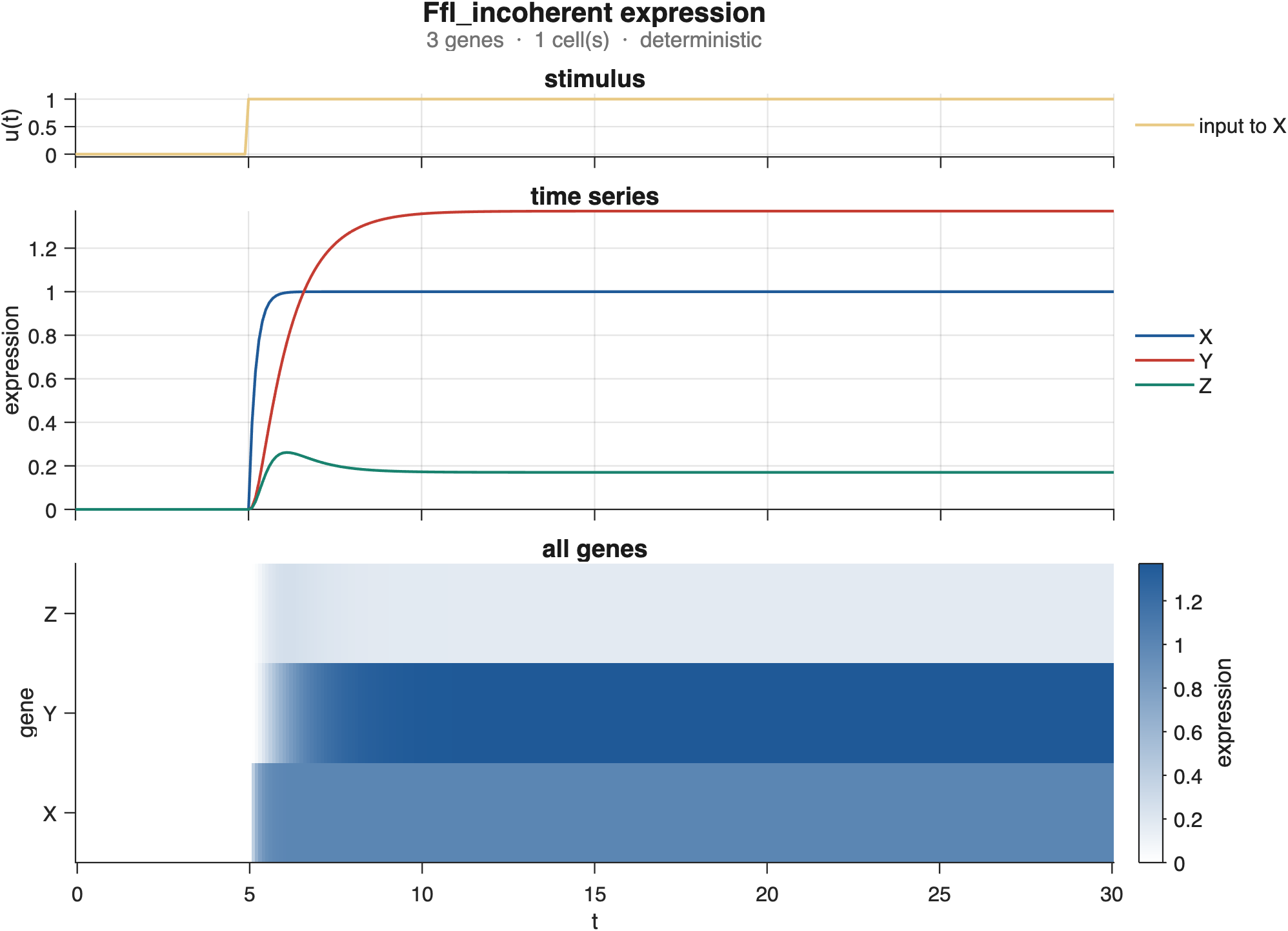
A single-input module driven from 0 to 3 times its normal rate. Left: steady-state dose response of the four targets, each with its own threshold and Hill coefficient. Right: the same information read dynamically from a slow ramp.

Example: the incoherent feed-forward loop pulse

model = grn.buildModel("ffl_incoherent", Logic = "multiplicative", Seed = 1, ...
    Params = struct("gamma", [5; 1; 3], "vmax", 5, "basal", [5; 0; 0]));
on  = grn.stimulus("X", "step", Baseline = 0, Amplitude = 1, Start = 5);
sol = grn.simulate(model, Stimulus = on, InitialCondition = zeros(3, 1), Duration = 30);
grn.plotExpression(sol);     % Z rises when X switches on, then Y catches up and represses it

The incoherent feed-forward loop with X switched on at t = 5. The top panel shows the input; Z pulses because X activates it directly before Y, which X also activates, arrives to repress it.

← Perturbations, steady states, and knockout screens Figures →