MATLAB · chapter 5 of 13

Simulating expression data

sol = grn.simulate(model, ...) integrates a model and returns a solution struct. model may be a model struct, a motif name, or a signed adjacency (the last two are built with grn.buildModel using the Logic and Seed you pass).

Time grid

Option	Default	Meaning
`Duration`	50	Recorded time span
`SampleDt`	0.1	Recording step; `sol.t = 0:SampleDt:Duration`
`Transient`	0	Time integrated and discarded before recording

Recording starts at t = 0. The transient, if any, runs at negative times, which matters for stimuli (their clock is sol.t).

Deterministic integration

Solver = "ode45" (default) or "ode15s". Both use RelTol = 1e-7, AbsTol = 1e-9, and MATLAB's NonNegative constraint on every state. ode15s receives the analytic Jacobian and is the better choice for stiff systems: widely different degradation rates, very high Hill coefficients, or two-stage models with slow proteins. The integration restarts at every stimulus edge, so step inputs are handled exactly rather than smeared across a solver step.

Cells and initial conditions

Option	Default	Meaning
`Cells`	1	Number of independent trajectories. `sol.x` becomes `samples x dim x Cells`
`RandomIC`	false	Draw each cell's initial state uniformly in `[0, scale]` per state
`InitialCondition`	`model.ic`	`dim x 1` shared by all cells, or `dim x Cells`

Cell k uses seed Seed + k - 1 for its initial condition and its process noise. With Cells > 1 and neither RandomIC nor Noise, every cell is identical; combine cells with random initial conditions, process noise, or both.

Perturbed genes (see Perturbations) have their random initial conditions scaled by the perturbation factor, so a knocked-out gene starts at zero.

sol = grn.simulate("repressilator", Cells = 20, RandomIC = true, Duration = 30, Seed = 3);
grn.plotExpression(sol, Cell = 1);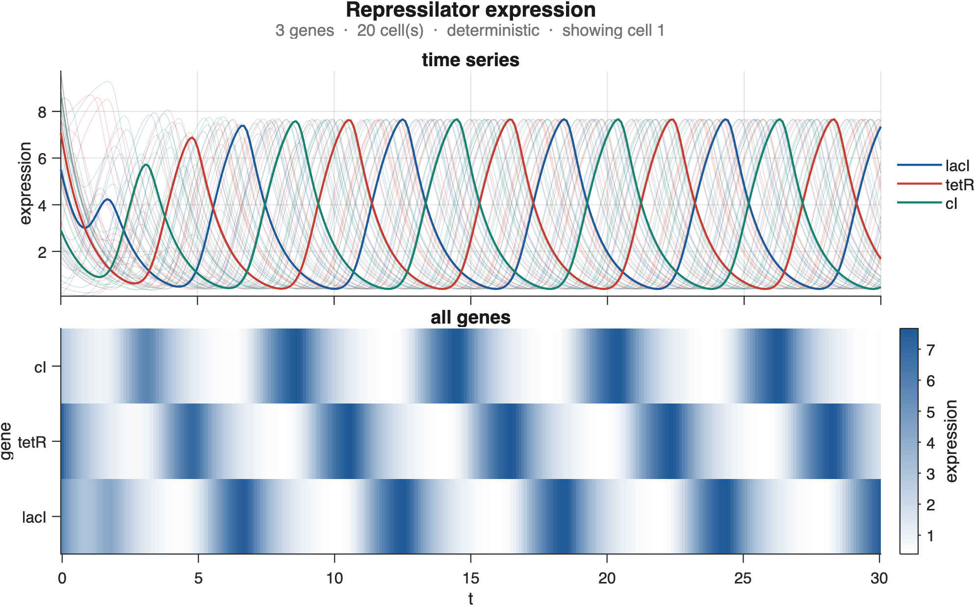

Twenty cells of the repressilator from random initial conditions. Cell 1 is drawn in full; the other 19 sit faintly behind it. Every cell oscillates with the same period but its own phase.

The same 20 cells: single traces on the left, the population mean on the right. Dephasing flattens the mean within two periods, which is exactly why bulk measurements of oscillating circuits look constant.

Process noise

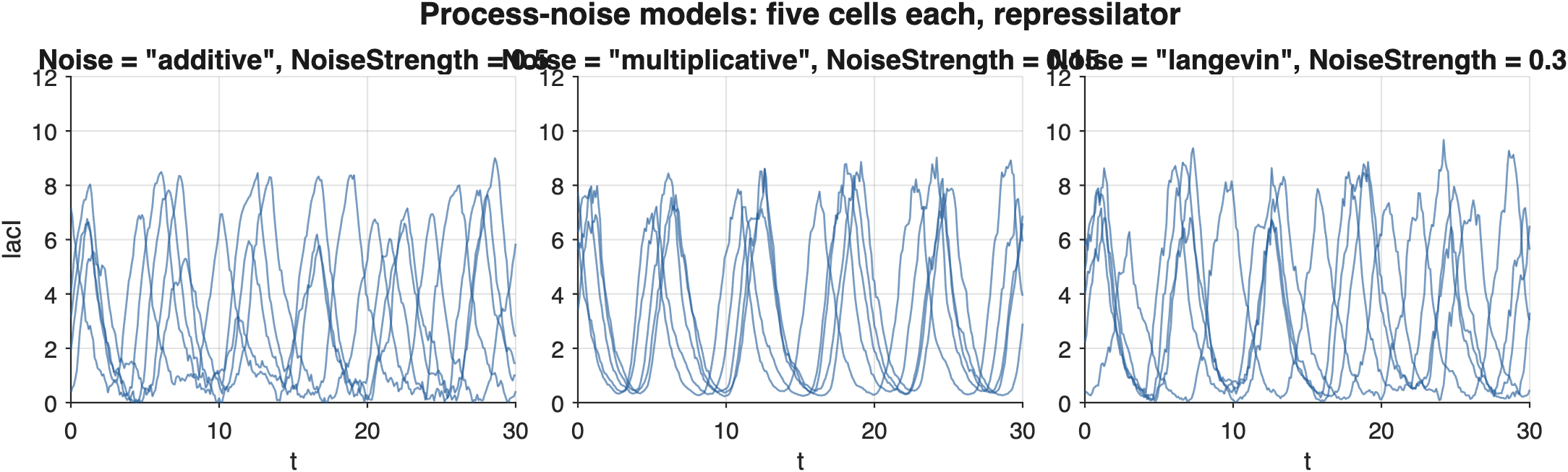
Noise switches from the ODE solvers to a fixed-step Euler–Maruyama integrator with step Dt (default SampleDt / 20; SampleDt must be an integer multiple of Dt). States are clipped at zero after every step.

`Noise`	Diffusion term per state	Use when
`"none"` (default)		Deterministic ODE
`"additive"`	`sigma`	Simple, level-independent fluctuations; the linear case has exact statistics
`"multiplicative"`	`sigma * x`	Fluctuations proportional to expression, never negative
`"langevin"`	`sigma * sqrt(birth + decay * x)`	Chemical Langevin equation: intrinsic noise from production and degradation events. `sigma` plays the role of `1 / sqrt(system size)`; the Fano factor of an unregulated gene equals `sigma^2`

NoiseStrength is sigma (default 0.1). For two-stage models the Langevin birth rate of an mRNA is its transcription rate and that of a protein is its translation rate.

The three process-noise models on the repressilator, five cells each. Additive noise jitters uniformly, multiplicative noise scales with expression, and the chemical Langevin form is quiet near zero and loudest at the peaks.

Observation noise

NoiseSigma adds Gaussian measurement noise after integration and clips at zero. It accepts a scalar, one value per gene (shared by that gene's mRNA and protein), or one value per state. The clean data are kept in sol.xClean.

Genetic perturbations and stimuli

Knockout, Knockdown, Overexpress, KnockdownFactor, OverexpressFactor are forwarded to grn.perturb; Stimulus is forwarded to grn.stimulate. See the next two chapters.

Reading the result

sol.t                 % samples x 1
sol.x                 % samples x dim [x cells]
sol.stateLabels       % names of the dim columns
sol.mrna, sol.protein % two-stage models only
sol.u                 % samples x n multiplicative input (all ones without stimuli)
sol.ic                % dim x cells initial conditions actually used
sol.options           % every option, with defaults filled in
sol.model             % the generating model

To stack all cells into one samples*cells x dim matrix (time within cell):

X = reshape(permute(sol.x, [1, 3, 2]), [], sol.dim);

A solution printed at the prompt:

sol = grn.simulate("repressilator", Cells = 4, RandomIC = true, NoiseSigma = 0.1)

Output

              t: [501×1 double]
              x: [501×3×4 double]
         xClean: [501×3×4 double]
          model: [1×1 struct]
              S: [3×3 double]
         labels: ["lacI"    "tetR"    "cI"]
    stateLabels: ["lacI"    "tetR"    "cI"]
              n: 3
            dim: 3
         stages: 1
          cells: 4
       stimulus: [0×0 struct]
              u: [501×3 double]
           uAdd: [501×3 double]
             ic: [3×4 double]
           type: "timeseries"
           name: "repressilator"
        options: [1×1 struct]

Choosing settings

Relaxation data (responses from random initial conditions): RandomIC = true, Duration around 5 to 10 mRNA lifetimes, no transient.
Stationary data (fluctuations around a steady state or oscillations): a Transient of at least 20 lifetimes, then a long Duration with process noise.
Single-cell-like ensembles: many Cells, RandomIC, Noise = "langevin", then keep one or a few time points per cell.
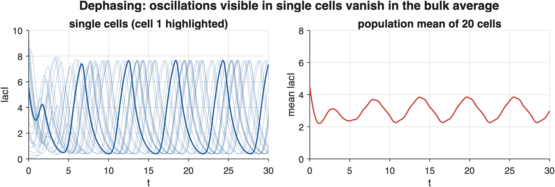
Bulk-like data: average sol.x over the cell dimension; oscillators dephase and average out, which is the correct behaviour.

Performance notes

Cost is linear in Cells and in Duration / Dt for stochastic runs. The multiplicative-logic Jacobian is O(n^3), which is only noticeable with ode15s above a few hundred genes. Deterministic runs of a 100-gene network take well under a second per cell.

← Building models Perturbations, steady states, and knockout screens →